HOE

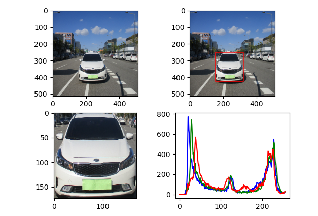
이전 장에서 학습한 2D histogram 분석을 이용해 여러 label 데이터의 분석을 진행하겠다 

1. image data

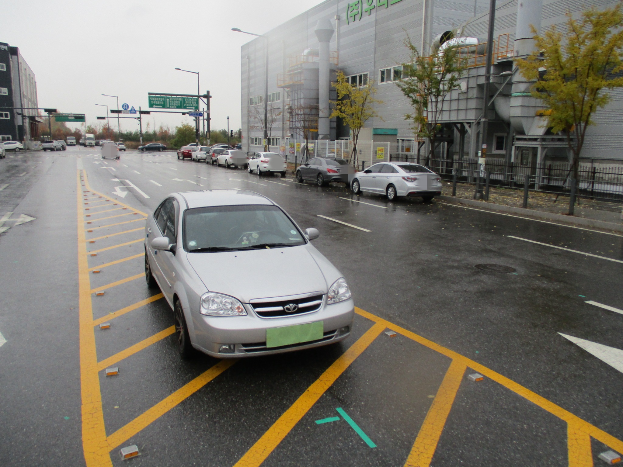
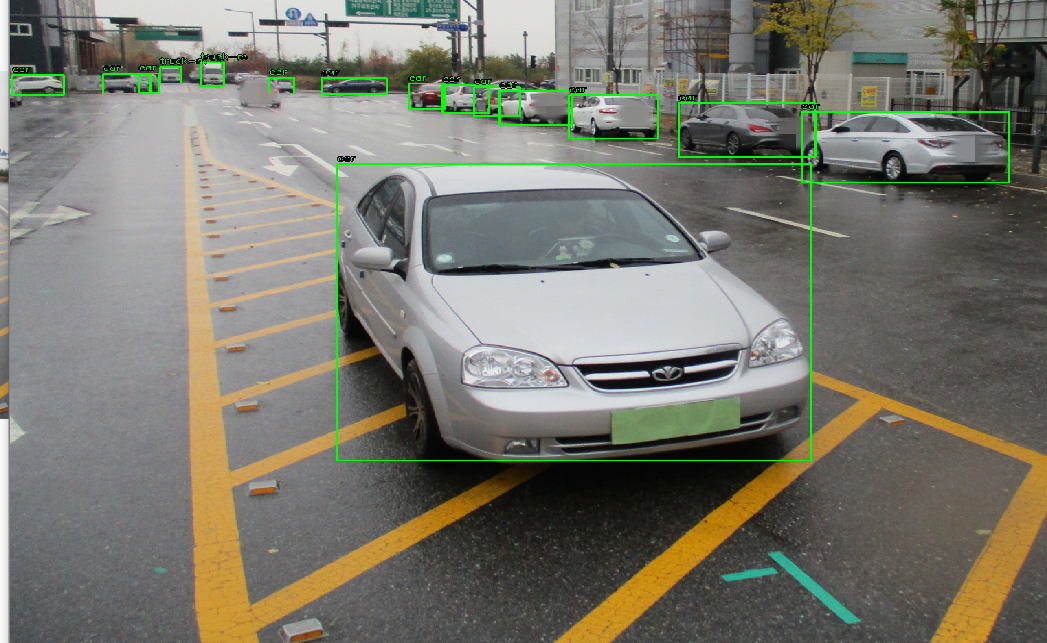
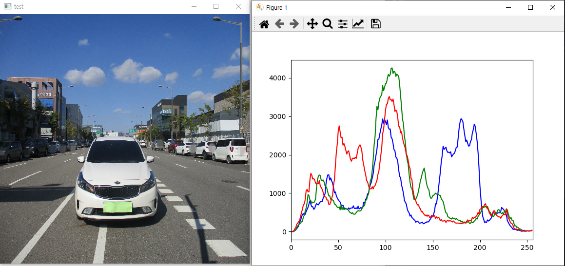
• 위의 사진을 보면 가운데 차량과 가상에 주차되어있는 차량에 바운딩박스가 쳐져 있다 
• 이 데이터를 가지고 각 각 바운딩 박스가 쳐져 있는 차량들의 2D histogram을 생성하여 어떤 분포를 가지고 있는지 비교하여 보겠다

import cv2
import numpy as np
import matplotlib.pyplot as plt

image = cv2.imread('test.JPG')
# hsv_image = cv2.cvtColor(image, cv2.COLOR_BGR2HSV)
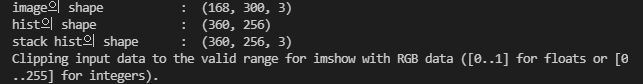
h,w,_ = image.shape
box_list = []
mask_image = []
temp_image = []
seed = 8
with open('test.txt','r') as rd:
    boxes = rd.readlines()
    for box in boxes:
        box = box.strip()
        box = box.split()
        box = list(map(float,box))
        box_width = box[3] * w
        box_height = box[4] * h
        box_center_x = box[1] * w 
        box_center_y = box[2] * h

        xmin = int(box_center_x - box_width/2)
        ymin = int(box_center_y - box_height/2)
        xmax = int(box_center_x + box_width/2)
        ymax = int(box_center_y + box_height/2)
        mask = np.zeros((h,w), np.uint8)
        mask[ymin:ymax, xmin:xmax] = 255 
        mask_image.append( cv2.resize(image[ymin:ymax,xmin:xmax],(300,300)))

for i in range(seed,len(mask_image)):
    if i == seed:
        temp_image = mask_image[i]
    else:
        temp_image = np.concatenate((temp_image,mask_image[i]), axis=1)
cv2.imshow('bounding boxes',temp_image)
cv2.waitKey(0)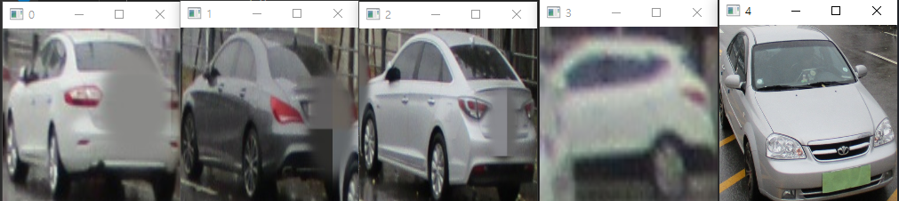

• 바운딩박스 영역의 객체들을 잘라내어 표시해 보았다 
• resize를 하여 2D histogram에 같은 비율로 적용이 되도록 하였다 
• 처음 알았는데 opencv imshow는 사용자의 해상도에 맞춰 이미지를 최대 해상도 까지만 표현한다 

2. cv2.compareHist(hist1, hist2, method)

• hist1 과 hist2 는 서로 비교할 histogram을 넣는다 
• method는 https://docs.opencv.org/3.4/d8/dc8/tutorial_histogram_comparison.html 에 공식까지 잘 나와있다 
  cv2.HISTCMP_CORREL : 두 히스토그램의 상관관계를 분석한다 
  cv2.COMP_CHISQR : 카이제곱검정으로 분석한다
  cv2.COMP_INTERSECT : Intersection 
  cv2.COMP_BHATTACHARYYA : bhattacharyya distance - 바타챠랴 거리 측정법으로 분석한다 hellinger distance와 같다
  cv2.COMP_KL_DIV : Kullback-leibler divergence - 쿨백-라이블러 발산으로 확률분포의 차이를 계산한다

import cv2
import numpy as np
import matplotlib.pyplot as plt

image = cv2.imread('test.JPG')
# hsv_image = cv2.cvtColor(image, cv2.COLOR_BGR2HSV)
h,w,_ = image.shape

mask_image = []
hist_list = []
with open('test.txt','r') as rd:
    boxes = rd.readlines()
    for i, box in enumerate(boxes[10:15]):
        box = box.strip()
        box = box.split()
        box = list(map(float,box))
        box_width = box[3] * w
        box_height = box[4] * h
        box_center_x = box[1] * w 
        box_center_y = box[2] * h

        xmin = int(box_center_x - box_width/2)
        ymin = int(box_center_y - box_height/2)
        xmax = int(box_center_x + box_width/2)
        ymax = int(box_center_y + box_height/2)
        mask = np.zeros((h,w), np.uint8)
        mask[ymin:ymax, xmin:xmax] = 255 
        add_image = cv2.resize(image[ymin:ymax,xmin:xmax], (200,200))
        cv2.imshow(str(i),add_image)
        add_image = cv2.cvtColor(add_image, cv2.COLOR_BGR2HSV)
        hsv_hist = cv2.calcHist([add_image],[0,1],None,[360,256],[0,360,0,256])
        cv2.normalize(hsv_hist,hsv_hist,0,1, cv2.NORM_MINMAX)
        hist_list.append(hsv_hist)
        

# cv2.compareHist
for i,hist1  in enumerate(hist_list):
    for j, hist2 in enumerate(hist_list):
        
        ret1 = cv2.compareHist(hist1,hist2, cv2.HISTCMP_CORREL)
        ret2 = cv2.compareHist(hist1,hist2, cv2.HISTCMP_CHISQR)
        ret3 = cv2.compareHist(hist1,hist2, cv2.HISTCMP_INTERSECT)
        ret4 = cv2.compareHist(hist1,hist2, cv2.HISTCMP_BHATTACHARYYA)
        ret5 = cv2.compareHist(hist1,hist2, cv2.HISTCMP_HELLINGER)
        ret6 = cv2.compareHist(hist1,hist2, cv2.HISTCMP_KL_DIV)
        print("\t\t\t\t\t\t\t{} 번과 {} 번의 비교".format(i,j))
        print("-------------------------------------------------------------------------------------------------------------------------------------------")
        print(" 상관관계 : {:.4f} \t 카이제곱 : {:.4f} \t 인터섹션 : {:.4f} \t 바타챠랴 : {:.4f} \t 헬링거 : {:.4f} \t 콜백발산 : {:.4f} ".format(
            ret1,ret2,ret3,ret4,ret5,ret6
        ))
        print("-------------------------------------------------------------------------------------------------------------------------------------------")
cv2.waitKey(0)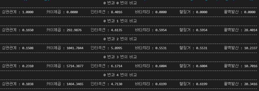

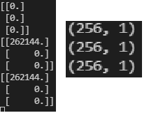
• calcHist로 계산한 결과를 normalize하여 0과 1의 값으로 보기 좋게 하였다 
• 바타챠랴 거리와 헬링거는 같은 함수이다 

https://github.com/dldidfh/tistory_code/tree/master/multi%20image%20histogram

이전 장에서 학습한 HSV포맷을 기준으로 2D Histogram 분석을 진행하겠다 

1. 2D Histogram 

• calcHist()  : 1D와 마찬가지로 calcHist 함수를 이용하여 HSV 포맷의 Hue와 Saturation의 histogram을 생성하겠다

from typing import no_type_check
import cv2
import numpy as np
from matplotlib import pyplot as plt

image = cv2.imread('test.jpg')
hsv_image = cv2.cvtColor(image, cv2.COLOR_BGR2HSV)
image = cv2.cvtColor(image, cv2.COLOR_BGR2RGB)
hist = cv2.calcHist(hsv_image,[0,1], None, [360,256], [0,360,0,256])
stack_hist = np.stack((hist,)*3,axis=-1)
print('image의 shape \t\t: ',image.shape)
print('hist의 shape \t\t: ',hist.shape)
print('stack hist의 shape \t: ',stack_hist.shape)

fig = plt.figure(figsize=(8,3))
plt.tight_layout()
plt.subplot((131)),plt.imshow(image)
plt.subplot((132)),plt.imshow(hist)
plt.subplot((133)),plt.imshow(stack_hist)

plt.show()

• 기존 1D Histogram을 그릴 때와 변경된 부분은
  4번째 파라미터인 x축 간격이 2개의 값을 넘겨 x와 y축으로 변경되었고
  5번째 파라미터인 축의 범위또한 x, y 각각 0~360 , 0~256의 범위로 설정되었다 
• 1D 일 때는 ply.plot으로 그래프를 그렸지만 2D에서는 imshow를 통해 보였다 그 이유는 1D에서는 각 그 값에 해당하는 픽셀의 개수를 표현했지만 2D에서는 H일 때 S 픽셀이 있나 를 표현해서 0, 1 의값이 리턴된다 그렇기 때문에 plot으로 2D를 그리면 0과 1만 표현된다 
• hist의 결과값은 H, S 2개의 값이 리턴되기 때문에 shape이 (360,256)이 된다 위에 가운데 사진에 보다시피 imshow로 보였을 때 잘 구분이 되지 않는다 
• 좀더 보기 쉽게 np.stack을 통해 RGB 같은 (360,256,3)의 shape으로 변경하였다
• 여기서 의문이 생긴다 각 값이 0과 1로 표현됐는데 왜 결괏값으로 보이는 이미지는 왜 검은색과 하얀색으로 표현되나 하얀색은 255가 아닌가? matplotlib.pyplot에서 0과 1로 되어있는 데이터는 자동으로 0,255로 변경해준다 

• 자 이제 나온 결과값을 해석해 보자 
• 세로의 값은 Hue를 뜻한다 (100,110) 정도에 점이 찍혀있다 그 뜻은 Hue:110, Saturation:100이란 뜻이므로 약간 어두운 초록색 부분이 많다는 뜻이다 사진에서 숲의 영역을 뜻한다
• 또한 H:160~250 S:150~200 까지의 부분에 점이 몰려있다 그 뜻은 밝은 하늘색이 다양한 밝기와 색상으로 존재한다는 뜻이다 사진에서 바다와 하늘을 뜻한다

다음장에서는 바운딩 박스를 읽어와

해당 바운딩박스 내에 객체들이

어떤 특성을 가지고 있는지 분석해 보겠다

이미지 형태, 비디오 형태의 분석을 위한 기초 분석 

1. cv2.calcHist(images, channels, mask, histSize, ranges)

• images : 분석 대상 이미지 (uint8 or float32) 
• channels : 분석 채널 grayscale은 [0], color는 [0],[0,1] : 1 Blue 2:Green 3: Red
• mask : 이미지의 분석 영역, None 은 전체 영역 
• histSIze : 분석 값 x축의 간격 하나의 
• range : x 축 범위  

import cv2
import os 
import numpy as np
from matplotlib import pyplot as plt

image = cv2.imread('test.jpg', cv2.IMREAD_COLOR)
image = cv2.resize(image, (512,512))
# image = cv2.cvtColor(image, cv2.COLOR_BGR2RGB)

# 0 : Blue, 1: Green, 2: Red
blue_hist = cv2.calcHist([image],[0],None,[256],[0,256])
green_hist = cv2.calcHist([image],[1],None,[256],[0,256])
red_hist = cv2.calcHist([image],[2],None,[256],[0,256])

plt.subplot(111), 
plt.plot(blue_hist , color='b'), 
plt.plot(green_hist, color='g'), 
plt.plot(red_hist, color='r'),

cv2.imshow('test',image)

plt.xlim([0,256])

plt.show()

• 위의 코드에서 주석처리된 부분에 cvt color 부분을 주석 처리한 이유는 opencv는 기본적으로 모든 색상 순서가 BGR로 되어있다. 그래서 변환 없이 바로 imshow로 보여주면 bgr을 bgr로 보여주기 때문에 cv2.imshow를 할 때는 ctvCOLOR를 이용할 이유가 없다. 하지만 plt.imshow()의 경우는 ctvCOLOR를 이용하여 보여줘야 원래 이미지대로 볼 수 있다. 
  
  

  

• 왼쪽은 cv2.imshow()를 한 이미지, 오른쪽은 plt.imshow()를 한 이미지 
• cv2.imshow는 BGR로 불러와 내보낼 때도 BGR로 내보내지만 cv2로 읽어온 객체를 plt로 내보내면 RGB 순서로 돼있
• 다는 가정하에 읽어오기 때문에 파란 이미지가 빨간색으로 표현된다 
  
  
  

  

• cv2.calcHist의 2번째 파라미터는 0: blue, 1:green, 2:red 이다 
• 각각 히스토그램의 shape를 찍어본 이유는 cv2.calcHist의 return value를 확인하기 위해서다. 각 1차원의 결괏값을 가진다 
  
  

• 다음과 같이 hist의 return 값은 x와 y 축의 2차원 배열이다 shape은 (256,1) 로써 첫 차원에는 0~ 255까지의 pixel의 개수가 포함되어 있다
• 왼쪽 사진은 위의 파란 이미지의 BGR 히스토그램 return값을 print 한것이다 
  Blue는 255 색상뿐이여서 0, 0, 0이라 나왔고 
  green과 red는 0 색상뿐이여서 배열의 첫 번째인 0 값이 해당 이미지의 넓이만큼 나왔다 ( 512x 512 = 262144 ) = blue는 모두 255이고 green, red는 모두 0이다라는 뜻 

2. calcHist mask 

• calcHist에 파라미터인 mask를 추가하여 특정 영역의 히스토그램을 추출할 수 있다 
• 차량의 레이블을 생성하여 읽어와 해당 레이블 영역의 히스토그램을 추출하여 보겠다 
  

  # print(image.dtype) : uint8
  mask = np.zeros(image.shape[:2], np.uint8)
  mask[box_ymin:box_ymax, box_xmin:box_xmax ] = 255
  
  mask_image = image[box_ymin:box_ymax, box_xmin:box_xmax]
  
  blue_hist = cv2.calcHist([image],[0],mask,[256],[0,256])
  green_hist = cv2.calcHist([image],[1],mask,[256],[0,256])
  red_hist = cv2.calcHist([image],[2],mask,[256],[0,256])
  
  plt.subplot(221),plt.imshow(image)
  plt.subplot(222),plt.imshow(testtestest)
  plt.subplot(223),plt.imshow(mask_image)
  plt.subplot(224), plt.plot(blue_hist, color='b'),plt.plot(green_hist, color='g'),plt.plot(red_hist, color='r')
  plt.xlim([-10,266])
  
  plt.show()​

• 기존의 calcHist 함수에 None으로 돼있던 위치에 mask 값을 추가하였다 
• mask 는 해당 이미지에서 추출할 영역을 선택한다 
• 중요한 점은 cv2.imread()로 읽어온 이미지는 uint8형 자료이기 때문에 mask를 적용할 때 mask의 값 또한 uint8로 맞춰줘야 한다 그렇기 때문에 mask = np.zeros()를 할 때 dtype=np.uint8로 지정하였다 

소스코드https://github.com/dldidfh/tistory_code/blob/master/%ED%9E%88%EC%8A%A4%ED%86%A0%EA%B7%B8%EB%9E%A8/histogram_opencv.py